Red Black Tree : An Intuitive Approach (A Deep Dive)
You can find the original writing in this GitHub Repo
Monologue
I remember when the first time I studied Red Black Tree (RBT) , it was an enigma . A seemingly random rotations and colorings seems to somehow balance a Binary Search Tree (BST) . But I had no intuition for why these rotations and colorings seem to magically balance the BST . I used to read these horrible case works and my reaction everytime after it got balanced was -

I had no idea what the RED and BLACK node represents . I didn’t even understand why they exist in the first place . After all , what has coloring got to do with the balancing of a Binary Search Tree , right ? . And why are they even called Red and Black , why not any other colors (the answer is hilarious XD) . All in all , it was a giant black box . All these Insert and Delete cases , nothing properly made sense . The number of unanswered questions stacked up and up . So , I had to do something about it . After few weeks of researching (read googling) , scouring through the internet and with a bit of imagination , I think I finally got ahold of the answers to all the questions that my dumb brain was unable to grasp : ) . This writeup is to accumulate all these answers and make an intuitive approach to Red BLack Trees so that dumb people like me can also have a proper intuition for the underlying operations in Red Black Tree and so that you don’t have to go through all of these by yourself again .
You might never need to understand the underlying intuitions behind all the operations . You can just call stl map or set in c++ and TreeMap in java , and can easily pass your life in peace . But if you do care for the intuition , you are in for a ride : D
The Story Begins
To properly understand anything one need to know its past . In my search for proper understanding of Red Black Trees , this is when it actually started to make sense to me for the first time .
I assume that you are familiar with Binary Search Trees and their shortcomings ( The complexity depends on tree height and in the worst case the height can be N , making most of the operations O(N) )
So , we need to somehow make it balanced such that on average the height is logN . Red Black Tree with it magic rotations and colorings seems to somehow do this . But this is not the only data structure to do this . The key to understanding RBT lies on the first few variant of this data structure that attempted to solve this balance of BSTs.
A slightly modified BST
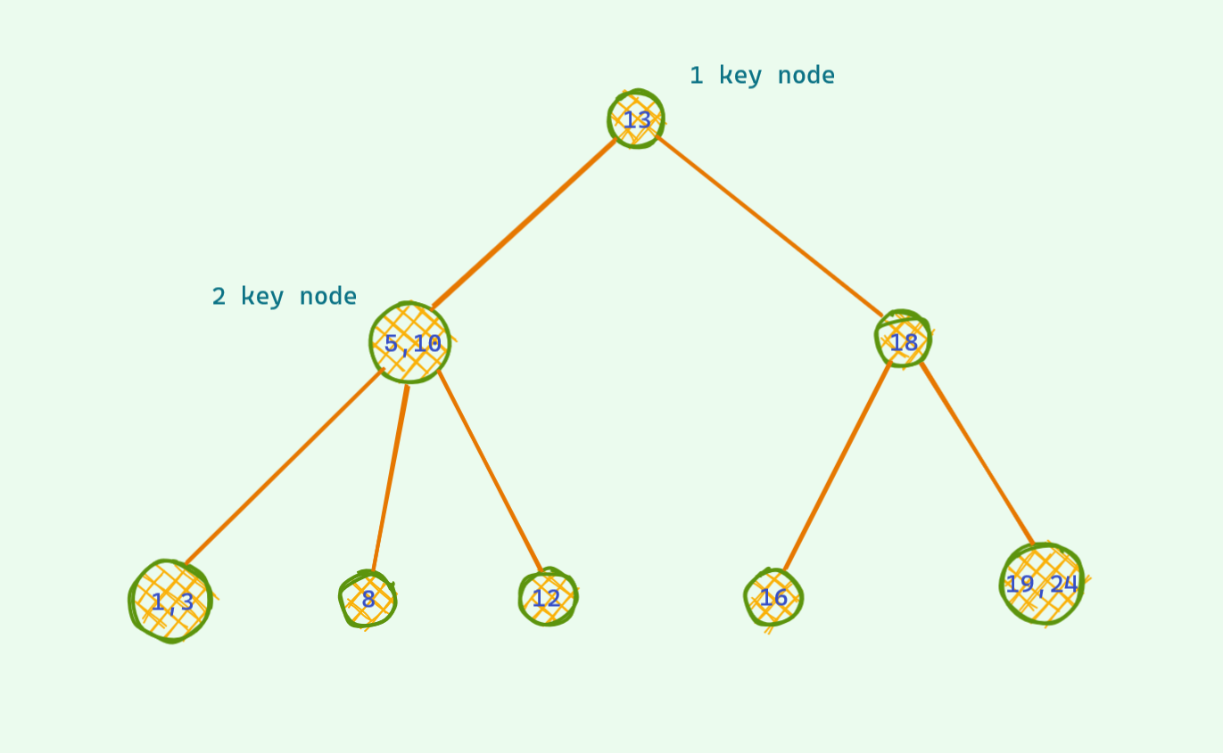
Let’s consider a slight variant of the BST. Instead of 1 key per node as in the regular BST , we will store upto 2 keys per node in this case and each node can have upto 3 child .
That’s it ! No other difference .
Now first consider insertion in this tree . How will we insert a node ?
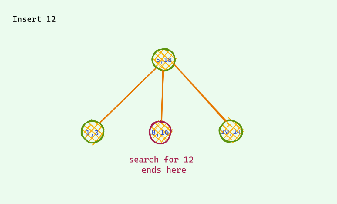
The idea is almost identical to regular BST . We compare the key wih the one in the tree and decide to go left , right or middle . Yes , the middle part is the only new thing here . This addition of new option is not hard to see why , since there can be 2 keys per node , the number of paths to take will be 3 of course !
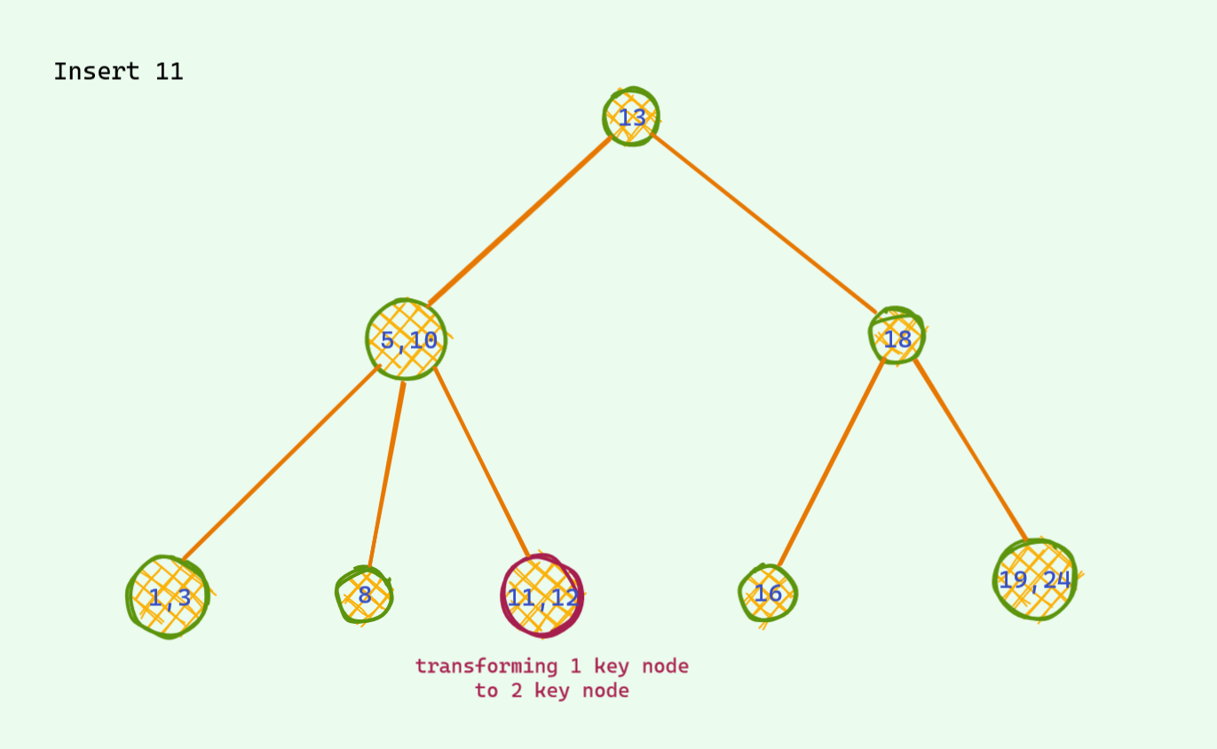
Now , what happens when we find the position for insertion key . If adding this key doesn’t change the property that we assumed (atmost 2 keys per node) , we can just easily add it !
When can we just add it without any concern ?
If we find that there is only 1 key , then we can just add another key and our tree properties will be perfectly fine !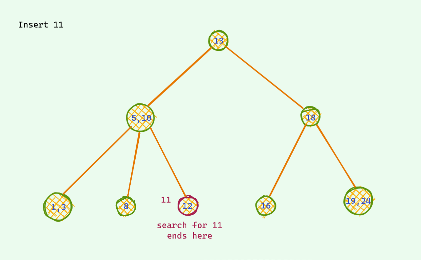
When does problem arise ?
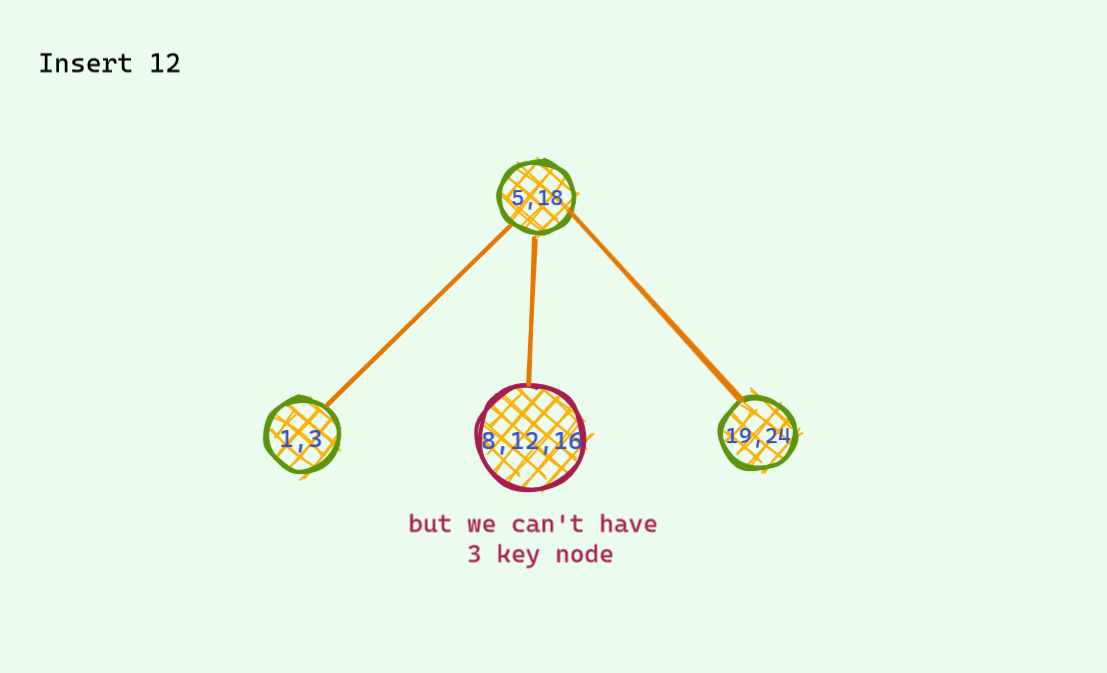
The problematic case : we find the corresponding place for insertion and we insert it . If after insertion we see there are 3 keys , we are in trouble : ( As mentioned earlier , there can be atmost 2 keys per node . So , we need to somehow fix this unstable node . Otherwise we are doomed . Here is an example .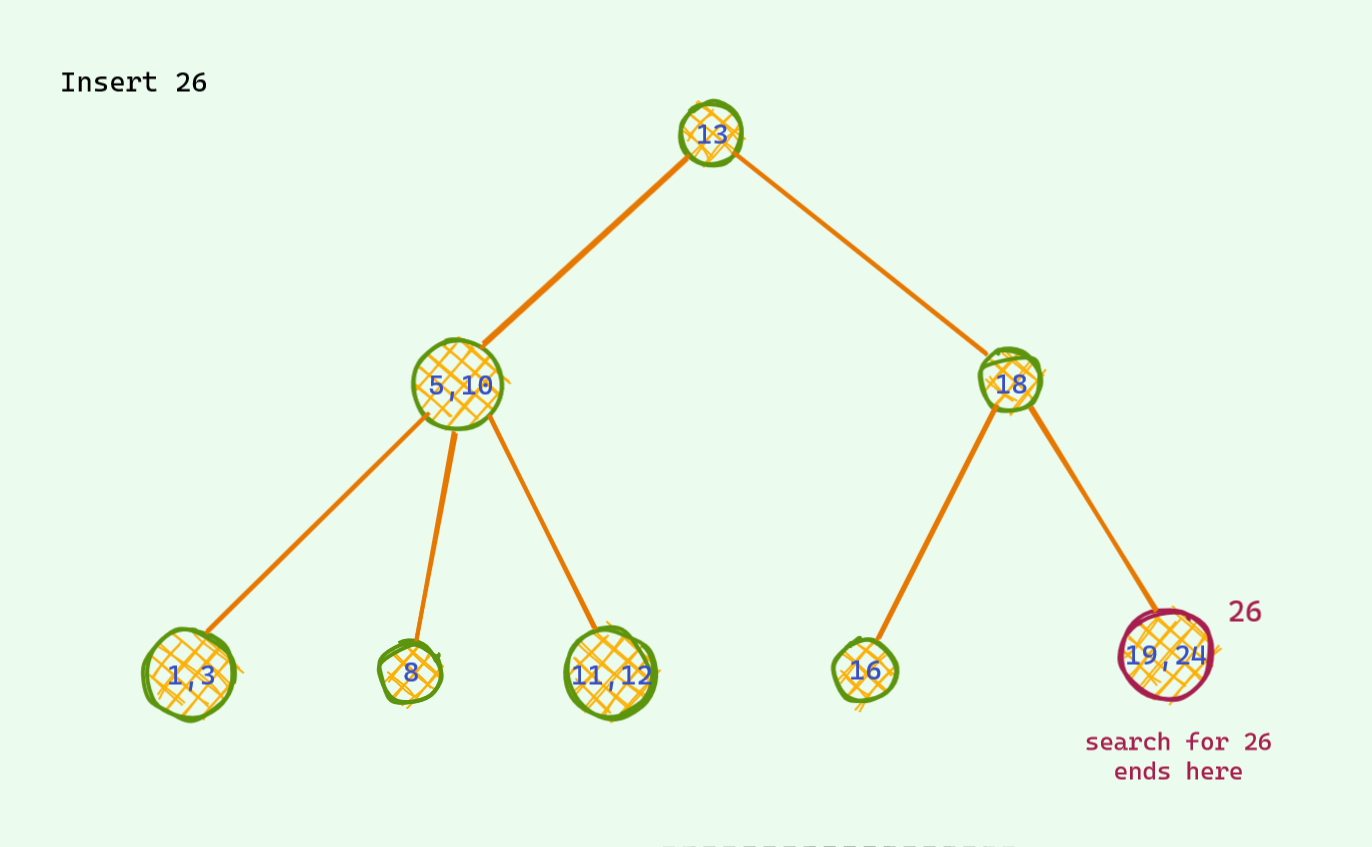
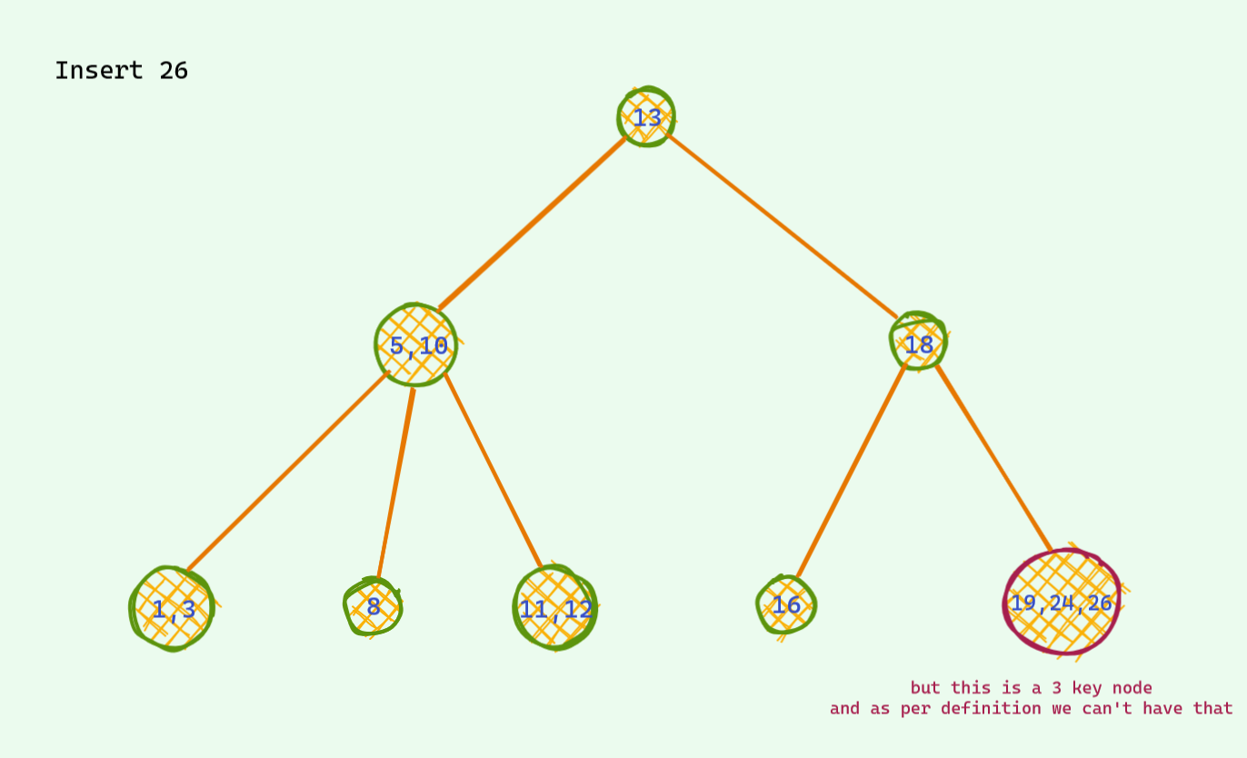
Now that we are stuck , it’s not hard no find a way around in this tree . We see that 18 is sitting lonely out there and has a place for one extra friend . We push up the middle key of the unstable node and voila we are good again . There are no more 3 key node in this tree .
Nice save : D
Now if you have good observation , you might have observed that all the leaf nodes have same distance from the root . This is not just a coincidence . Let’s see why this is the case .
We have seen 2 different type of insertions so far and if you noticed , none of them changed the height of the tree . Now let’s consider a case where the push up is such that there is an increase of height .
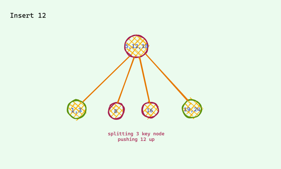
Did you see what just happened ? The height of the tree increased by 1 and the distance of all the leaf nodes increased exactly by 1 . Thus leading to having all the leaf nodes in the same height/depth .
Key Takeaway from slightly modified BST
We saw earlier that if there was a way to balance our BST , we can efficiently do operations . Our slightly modified BST does exactly that ! We just saw that our tree is always perfectly balanced !
In this slightly modified BST ,
- Worst Case Height :
O(log_base2_N)/O(logN)(All nodes have 2 keys) - Best Case Height :
O(log_base3_N)(All nodes have 3 keys)
Modifying one step further
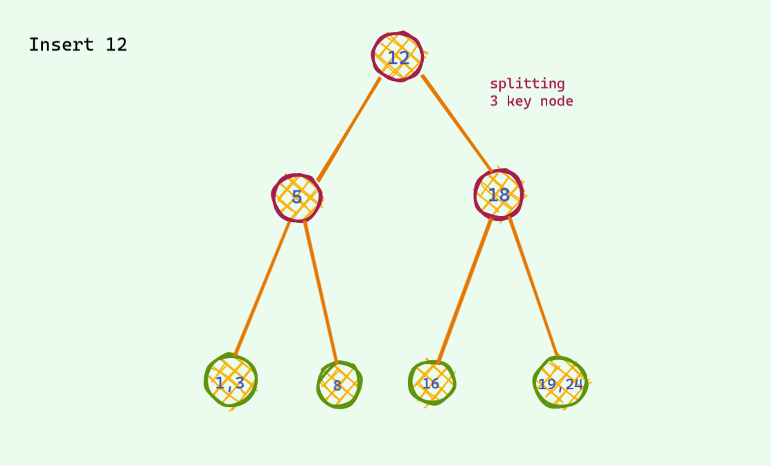
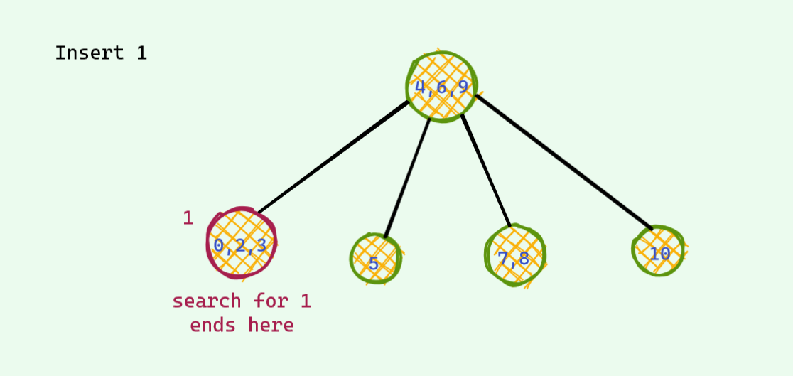
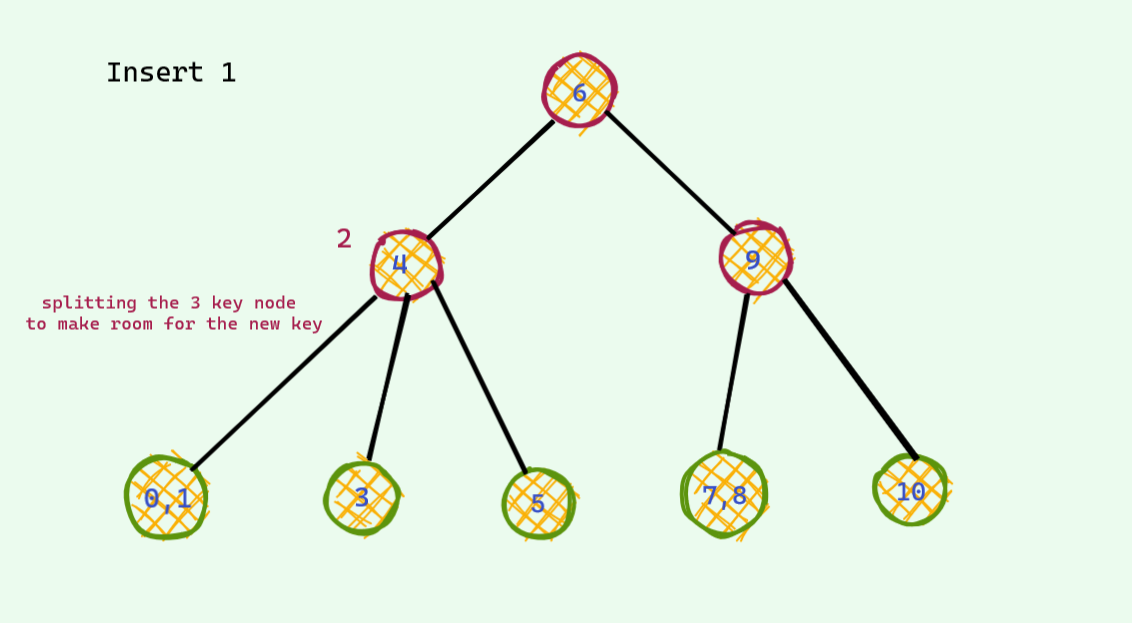
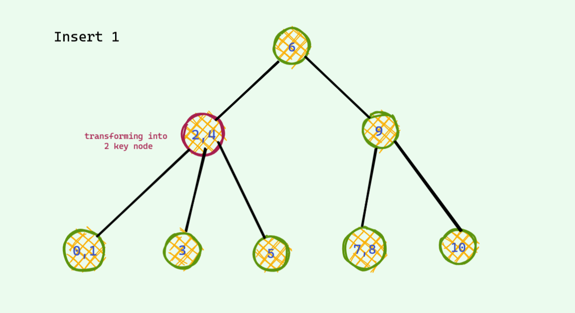
This time we will allow upto 3 keys per node . One more than the last time . This time there is also one problematic case : when we have 4 keys per node . We also do almost the same thing we did the last time . When there is a potential 4 key node , we split to make room for the new key .
I will just show an example and won’t dive deep .

Changing Vantage Point
Simulating this tree seems to be very easy in hand . But coding up this is not . Maintains variable number of keys in a node and also handling tree splitting can be a cumbersome job to do . If you are a lazy guy like me you wouldn’t dare to implement this .
Now , let’s change our vantage point . Let’s cleverly represent this nodes so that we don’t have to deal with all these tree splitting and variable nodes .
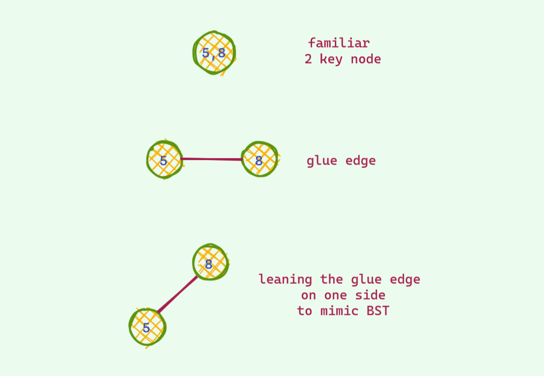
With a bit of imagination , we can think the 2 key nodes as 2 separate nodes glued together by an edge . If we draw this link by leaning on the side a bit , you can see that it is just your familiar BST .
But wait ! How do you distinguish between an ordinary edge and a glue edge . Yes ! we color it : D
Here’s how we can represent the 2 key nodes :
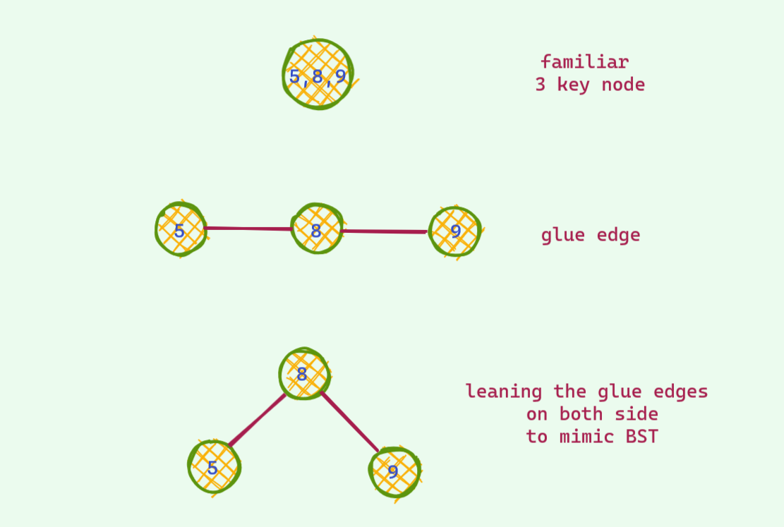
And here’s how we can represent the 3 key nodes :
We can also instead color children nodes thus making it convenient to implement as tracking edge colors in BST implementation would not be a headache anymore .
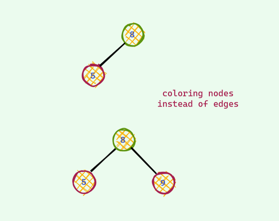
This was the eureka moment for me ! This is the Red Black Tree we have studied blindly all this time ! Finally we figured out the coloring ! RBT is nothing but a fancy way of representing the modified BSTs we saw earlier . Isn’t this great ? : D

Now you ask , why is this red ? Why not any other colors ?
Answer
It was because the guys who invented this , only had red and black pens to draw :v And they chose to color the nodes red .
Inside the Black Box
Insert
Now , we know that the operations we saw till now was RBT under the hood . Let’s see how these operations look in the RBT .
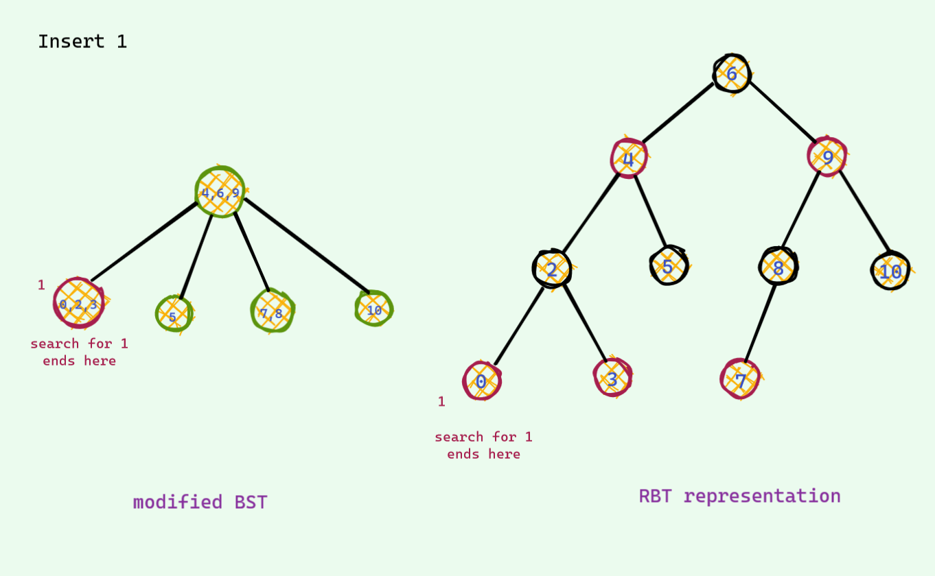
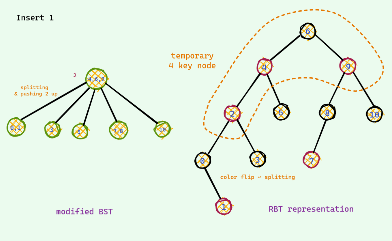
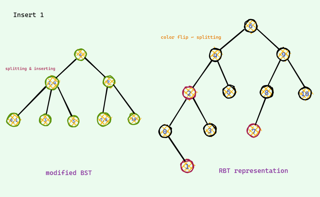
If you open a random book , you must have seen this weird rule which goes something like this : when there are 2 red nodes in a row and uncle is also a red node , we do color flip . Now you see what those color flip actually do ! These is just a fancy way to implement the splitting on the modified BST .
Now , let’s see another type of insertion .
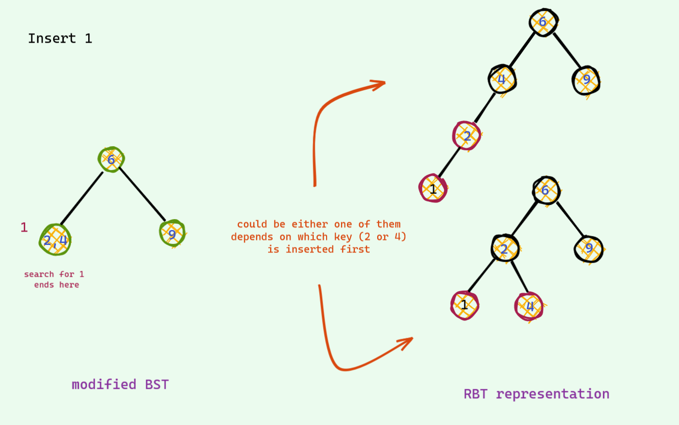
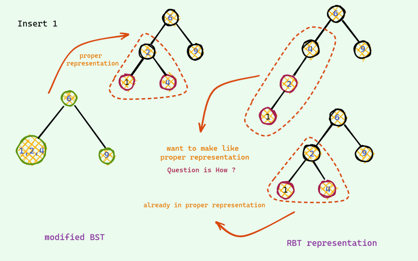
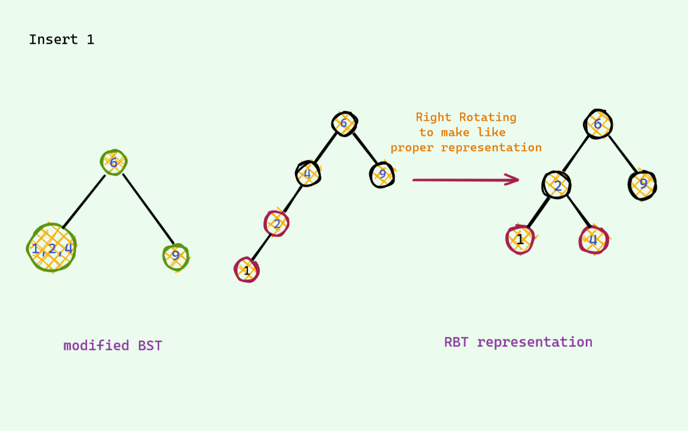
You might have also seen a rule which goes something like this : _when there are 2 red nodes in a row and uncle is a black node , we need to rotate to balance the RBT _. This is just a normal insertion in the modified BST ! This one has 2 case : the node could be red nodes could be in Left Right order unlike the Left left order shown in the last example . This is the same , we just do 2 rotations to come to our proper 3 key node representation .
Delete
Insertion was pretty easy . Most of the books represent delete in RBT as an awful hard operation . Infact when I first read the deletion , it was just a bunch of messy casework to memorize and I had no idea what the heck we were actually doing . But now , it has changed . Deletion is not difficult than insertion in any way , if not easier !
But , first let’s recap some RBT properties which can be easily seen from our modified BST analogy :
- In modified BST , all leaf nodes were at the same height . So , in our RBT all the subtrees will have same black height (remember how red nodes doesn’t contribute to the height , we just lean on either side to mimic BST)
- Root is always black
This 2 properties are enough to understand Deletion .
Deletion process is almost similar to the normal BST . I won’t dive deep . Here is a recap :
- If we have less than 2 child , we can delete this node
- Otherwise , we replace with the successor / predecessor node and delete that node instead
Now in case of RBT , there can be some violation . Let’s see :
- If we are deleting a red node , we are safe (Remember that we can easily delete from 2 key node in our slightly modified BST as it doesn’t affect the height of the tree)
- But if we are deleting a black node , we are in trouble : ( Deleting a black node will violate the first property we have seen earlier . We gotta fix this . This is the whole fiasco is about .
Let’s begin . Rather than telling you a bunch of awful rules to memorize , let us see what can and can’t be done intuitively . Let me walk you thorough -
The Easy One
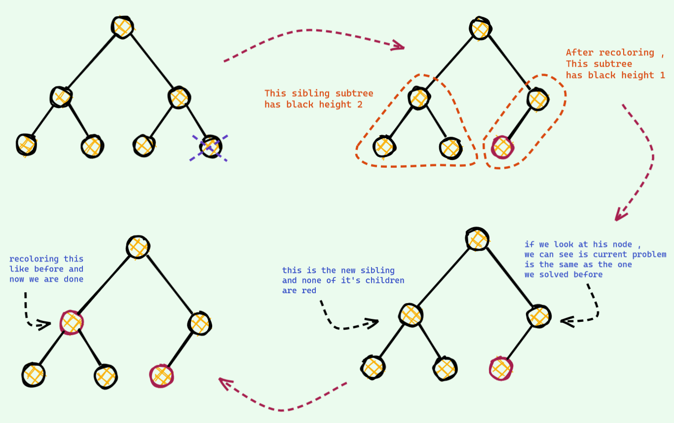
This time , the node we deleted has black sibling and no red children . Let see how it goes if we want to restore balance -
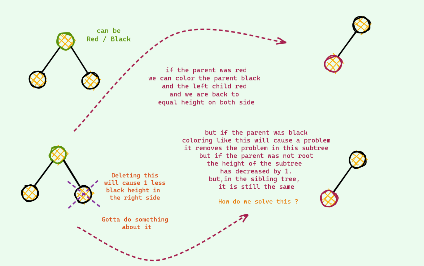
The idea to solve this is we hand our problem to the parent . And if the parent couldn’t solve , then we repeat the same process . We know that it will be fixed some time in the future because we just saw in the case of parent being the root , our problem is solved immediately .
The Easier One
This time , the node we deleted has black sibling and at least one red children . Let’s see how this one goes -
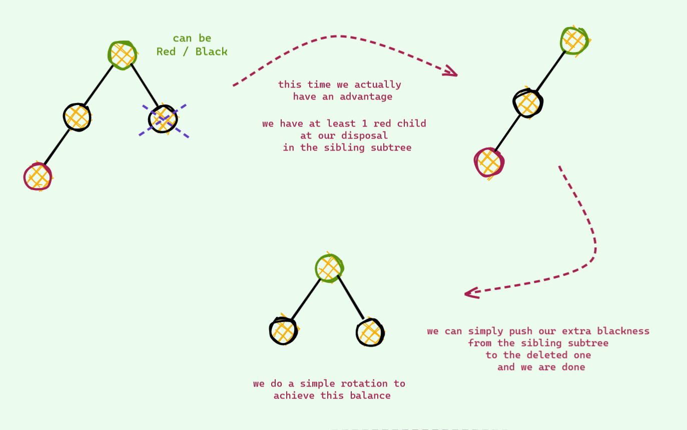
Pretty easy !
There is just one corner case , if the only red child was the right node in the example we just saw , we would have to do one more rotation (like we did in the insert) to make it like the one we solved .
The Clever One
We are almost done . We just need to take care of one last thing . The red sibling case -
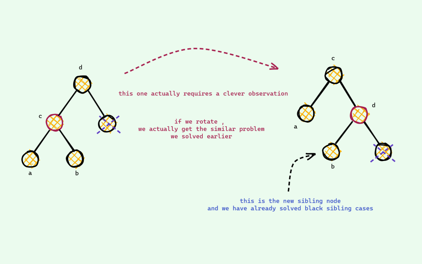
And now , we are done . See ! It was not that bad . Once we know why we are doing what , it immensely simplifies stuffs !
Getting our hands dirty (with code)
All these efforts till now were all for this . We had to come up with glue nodes and colorings and what not just so that we can easily implement this thing . So , let’s get into it !
I remember when i first the RBT pseudocode from Cormen (CLRS) , I had a mini heart attack . My first reaction was , “ Eww, how can a code be this ugly ! “ And the impression hasn’t changed a bit . It is still one of the most ugliest implementation I’ve seen till date . Coding a red black tree doesn’t have to be this ugly .
Instead , I will guide you with a recursive implementation which I found much easier to code . Much much easier to debug and the size of the code will be half the size of the cormen implementation if not less .
The Node
We need just one more information from our usual BST : Color . No need to track parent or any other things . And about why we have taken a pointer array , not 2 left right pointers , I will get to that in a second .
1 |
|
Auxiliary Operations
The main auxiliary operations are rotation and color flipping . The implementations are pretty much straightforward . If we had taken 2 separate pointers , the implementation would be like this
1 | void colorFlip(Node *node) |
But , if instead we had implemented using pointer array , we can actually write only one function for the rotation !
1 | Node* rotate(Node *node,bool dir) /// direction : left / right |
And this way , our double rotation code is just 2 lines !
1 | Node* doubleRotate(Node *node,bool dir) /// align reds , then rotate |
We have already made our code half the size ! You will be amazed to see the magic of this further when we don’t have to seperately handle the mirror cases in insert and delete operation : D At least I was , when I found out this trick when scouring through the internet which dramatically reduced my original insert implementation .
Let’s get into insertion .
Insert
1 | void insert(int data) |
We just need to write this magic function INSERT_FIX_UP and we are done ! Iterative implementations needs to track parent and also handing all the cases can be really pain . But , we will take advantage of the bottom up approach . If a RBT property violation has occurred , we will fix on our way up in the recursion !
1 | Node* INSERT_FIX_UP(Node *node,bool dir) |
See , how we don’t need to write code for additional mirror cases !
Delete
The delete skeleton is the same as regular BST , with just one minor change . We keep a flag variable to keep track if we have already restored the balance or not .
1 | void delete_(int data) |
Now , we have to write the magic function DELETE_FIX_UP .
1 | Node* DELETE_FIX_UP(Node *node,bool dir, bool &ok) |
Ah , we are done finally ! It was not that awful , was it ?
Optimization and Conclusion
If you have come this far down , let me tell you one more thing . The RBT we studied is the classical old RBT . There are other implementations of RBT which makes the code even more shorter and easier to write . Among these , one is Left Leaning Red Black Tree (LLRB) . It is nothing but the implementation of the first modified BST we saw . And about the implementation , we can also use a topdown approach , that is also easier to understand than the bottom up approach . If you do feel interested , check them out .
Congrats on reading this far : D If you have any problem , do let me know . And if you liked the writeup do let me know too !
Reference
Ah! lot of them , I’m going to mention as many as I can remember.
- https://en.wikipedia.org/wiki/Red%E2%80%93black_tree?oldformat=true
- https://www.cs.purdue.edu/homes/ayg/CS251/slides/chap13c.pdf
- http://smile.ee.ncku.edu.tw/old/Links/MTable/Course/DataStructure/2-3,2-3-4&red-blackTree_952.pdf
- https://stackoverflow.com/questions/15455042/can-anyone-explain-the-deletion-of-left-lean-red-black-tree-clearly
- https://www.cs.princeton.edu/~rs/talks/LLRB/LLRB.pdf
- https://stackoverflow.com/questions/364616/in-red-black-trees-is-top-down-deletion-faster-and-more-space-efficient-than-bot/8024168#8024168
- https://www.youtube.com/watch?v=DQdMYevEyE4
- https://eternallyconfuzzled.com/red-black-trees-c-the-most-common-balanced-binary-search-tree
- https://stackoverflow.com/questions/14119995/red-black-tree-top-down-deletion-algorithm?rq=1
- https://stackoverflow.com/questions/13360369/deletion-in-left-leaning-red-black-trees
- ftp://ftp.cs.princeton.edu/techreports/1985/006.pdf
- https://sites.cs.ucsb.edu/~teo/cs130a.m15/rbd.pdf
- https://stackoverflow.com/questions/14119995/red-black-tree-top-down-deletion-algorithm
- https://iq.opengenus.org/red-black-tree-deletion/
- https://github.com/jeffrey-xiao/competitive-programming/blob/master/src/codebook/datastructures/RedBlackTree.java
- https://www.topcoder.com/community/competitive-programming/tutorials/an-introduction-to-binary-search-and-red-black-trees/
- https://softwareengineering.stackexchange.com/questions/141834/how-is-a-java-reference-different-from-a-c-pointer
- https://www.programiz.com/dsa/red-black-tree
- https://www.cs.usfca.edu/~galles/visualization/RedBlack.html
- https://www.cs.princeton.edu/courses/archive/fall06/cos226/lectures/balanced.pdf
- https://www.cs.princeton.edu/courses/archive/spring19/cos226/lectures/33BalancedSearchTrees.pdf